Peak-Set Enrichment Analysis with PeakSEA

Introduction

What is PeakSEA?

Peak-Set Enrichment Analysis (PeakSEA) is a computational method for identifying which peak sets — collections of genomic regions sharing a biological property — are over-represented among peaks that are differentially regulated between conditions.

PeakSEA adapts the Gene Set Enrichment Analysis (GSEA) framework (Subramanian et al., 2005) to genomic ranges data. The key conceptual differences are:

GSEA	PeakSEA
Input: genes ranked by differential expression	Input: peaks ranked by differential accessibility
Gene sets (e.g. GO terms, pathways)	Peak sets (e.g. ATAC peaks, DHS, histone marks)
Membership defined by gene identifier	Membership defined by genomic coordinate overlap

The approach can for example be applied to chromatin accessibility experiments where one wishes to ask: “Do peaks near binding sites of TF X tend to be more open in condition A?”

Algorithm overview

Ranked peaks (gr)               Peak set database (gr_set)
  chr1:1000-1499  log2FC=3.1        chr1:1050-1550  term="CTCF"
  chr1:2000-2499  log2FC=2.7    ──► chr1:2100-2600  term="CTCF"
  chr2:500-999    log2FC=-1.2       chr3:800-1300   term="H3K27ac"
  ...                               ...
        │
        │  1. Overlap peaks with peak sets
        ▼
  Annotate each peak with the term(s) it overlaps
        │
        │  2. Build ranked gene-set input for GSEA
        ▼
  TERM2GENE data frame  +  named ranked vector
        │
        │  3. Run GSEA (clusterProfiler)
        ▼
  gseaResult: NES, p-value, FDR per peak set

Input data

Ranked peaks (`gr`)

gr must be a GRanges object whose metadata contains a quantitative ranking metric. Common choices:

log2FC from a differential accessibility test (e.g. DESeq2, edgeR)
Signed $-\log_{10}(p\text{-value})$
Any continuous score where larger values indicate stronger signal in the condition of interest

library(PeakSEA)
library(plyranges)

set.seed(1979)

# 100 simulated ATAC-seq peaks with strong signal:
#   peaks 1–50 are upregulated (positive log2FC)
#   peaks 51–100 are downregulated (negative log2FC)
peaks <- data.frame(
  seqnames = "chr1",
  start    = seq(1e4, by = 1e3, length.out = 100),
  width    = 500L,
  log2FC   = c(seq(5, 0.1, length.out = 50),
               seq(-0.1, -5, length.out = 50)),
  padj     = runif(100, 0, 0.05)
) |>
  plyranges::as_granges()

peaks
#> GRanges object with 100 ranges and 2 metadata columns:
#>         seqnames        ranges strand |    log2FC       padj
#>            <Rle>     <IRanges>  <Rle> | <numeric>  <numeric>
#>     [1]     chr1   10000-10499      * |       5.0 0.04544498
#>     [2]     chr1   11000-11499      * |       4.9 0.02410026
#>     [3]     chr1   12000-12499      * |       4.8 0.01264799
#>     [4]     chr1   13000-13499      * |       4.7 0.03642297
#>     [5]     chr1   14000-14499      * |       4.6 0.00827964
#>     ...      ...           ...    ... .       ...        ...
#>    [96]     chr1 105000-105499      * |      -4.6  0.0119499
#>    [97]     chr1 106000-106499      * |      -4.7  0.0375665
#>    [98]     chr1 107000-107499      * |      -4.8  0.0201940
#>    [99]     chr1 108000-108499      * |      -4.9  0.0232156
#>   [100]     chr1 109000-109499      * |      -5.0  0.0108765
#>   -------
#>   seqinfo: 1 sequence from an unspecified genome; no seqlengths

Peak set database (`gr_set`)

gr_set is a GRanges object where every range is annotated with a "term" metadata column naming the peak set it belongs to. This mirrors the TERM2GENE format used by clusterProfiler.

Peak sets can represent, for example:

TF binding sites from ChIP-seq experiments (ENCODE, ReMap)
Chromatin states from histone mark ChIP-seq (Roadmap Epigenomics)
DHS clusters from DNase-seq
Any custom collection of genomic intervals

Public databases such as LOLA and AnnotationHub provide pre-built region sets that can be used directly as gr_set.

For this vignette we create two synthetic peak sets that mimic TF binding sites overlapping a known subset of our differential peaks:

# "TF_A" binding sites overlap the upregulated peaks
# "TF_B" binding sites overlap the downregulated peaks
set.seed(1979)
peak_sets <- c(
  shift_right(peaks[sample(1:60, 40)],  100L) |> mutate(term = "TF_A"),
  shift_right(peaks[sample(40:100, 40)], 100L) |> mutate(term = "TF_B")
)

peak_sets
#> GRanges object with 80 ranges and 3 metadata columns:
#>        seqnames      ranges strand |    log2FC      padj        term
#>           <Rle>   <IRanges>  <Rle> | <numeric> <numeric> <character>
#>    [1]     chr1 55100-55599      * |       0.5 0.0270753        TF_A
#>    [2]     chr1 46100-46599      * |       1.4 0.0462161        TF_A
#>    [3]     chr1 11100-11599      * |       4.9 0.0241003        TF_A
#>    [4]     chr1 68100-68599      * |      -0.9 0.0210772        TF_A
#>    [5]     chr1 41100-41599      * |       1.9 0.0348013        TF_A
#>    ...      ...         ...    ... .       ...       ...         ...
#>   [76]     chr1 56100-56599      * |       0.4 0.0308319        TF_B
#>   [77]     chr1 60100-60599      * |      -0.1 0.0212098        TF_B
#>   [78]     chr1 50100-50599      * |       1.0 0.0279952        TF_B
#>   [79]     chr1 69100-69599      * |      -1.0 0.0120466        TF_B
#>   [80]     chr1 98100-98599      * |      -3.9 0.0105650        TF_B
#>   -------
#>   seqinfo: 1 sequence from an unspecified genome; no seqlengths

Running PeakSEA

Call psea() with the ranked peaks, the name of the ranking column, and the peak set database. Additional arguments are forwarded to plyranges::join_overlap_left() (e.g. maxgap, minoverlap) to control how overlaps between gr and gr_set are computed.

result <- psea(peaks, log2FC, peak_sets)

result
#> #
#> # Gene Set Enrichment Analysis
#> #
#> #...@organism     unknown 
#> #...@setType      unknown 
#> #...@keytype      unknown 
#> #...@geneList     Named num [1:100] 5 4.9 4.8 4.7 4.6 4.5 4.4 4.3 4.2 4.1 ...
#>  - attr(*, "names")= chr [1:100] "chr1_10000_10499" "chr1_11000_11499" "chr1_12000_12499" "chr1_13000_13499" ...
#> #...nPerm     1000 
#> #...pvalues adjusted by 'BH' with cutoff < 0.05
#> #...2 enriched terms found
#> 'data.frame':    2 obs. of  12 variables:
#>  $ ID             : chr  "TF_B" "TF_A"
#>  $ Description    : chr  "TF_B" "TF_A"
#>  $ setSize        : int  40 40
#>  $ enrichmentScore: num  -0.759 0.719
#>  $ NES            : num  -3.03 2.83
#>  $ pvalue         : num  1.62e-10 4.44e-09
#>  $ p.adjust       : num  3.25e-10 4.44e-09
#>  $ qvalue         : num  NA NA
#>  $ rank           : int  45 42
#>  $ leading_edge   : chr  "tags=80%, list=45%, signal=73%" "tags=72%, list=42%, signal=70%"
#>  $ core_enrichment: chr  "chr1_66000_66499/chr1_67000_67499/chr1_68000_68499/chr1_69000_69499/chr1_71000_71499/chr1_72000_72499/chr1_7300"| __truncated__ "chr1_10000_10499/chr1_11000_11499/chr1_12000_12499/chr1_13000_13499/chr1_14000_14499/chr1_16000_16499/chr1_1800"| __truncated__
#>  $ log2err        : num  0.827 0.761
#> #...Citation
#> S Xu, E Hu, Y Cai, Z Xie, X Luo, L Zhan, W Tang, Q Wang, B Liu, R Wang, W Xie, T Wu, L Xie, G Yu. Using clusterProfiler to characterize multiomics data. Nature Protocols. 2024, 19(11):3292-3320

The result is a gseaResult object. The embedded result table can be accessed as a data frame:

knitr::kable(as.data.frame(result)[, c("ID", "NES", "pvalue", "p.adjust")])

	ID	NES	pvalue	p.adjust
TF_B	TF_B	-3.026348	0	0
TF_A	TF_A	2.833434	0	0

Interpreting the output:

NES > 0: the peak set is enriched among upregulated peaks (top of the ranked list).
NES < 0: the peak set is enriched among downregulated peaks (bottom of the ranked list).
p.adjust: FDR (Benjamini–Hochberg by default).

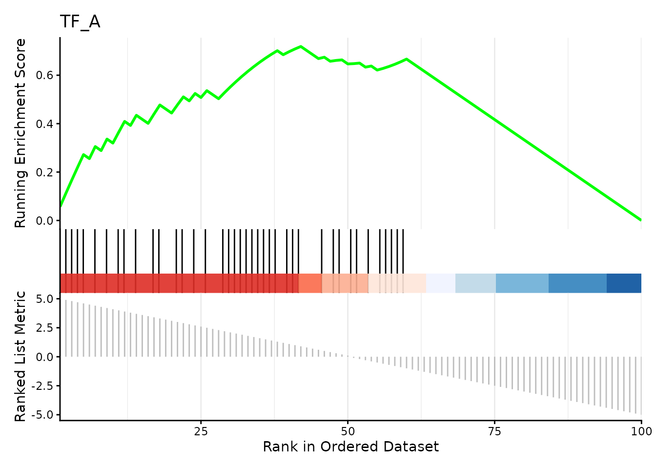
As expected, TF_A (associated with upregulated peaks) has a positive NES, while TF_B (associated with downregulated peaks) has a negative NES.

Visualisation

enrichplot provides ready-made plots for gseaResult objects.

The enrichment curve for an individual peak set shows how its members are distributed across the ranked peak list:

if (requireNamespace("enrichplot", quietly = TRUE)) {
  enrichplot::gseaplot2(result, geneSetID = "TF_A", title = "TF_A")
}

Building a peak set database from public resources

In a real analysis, gr_set is typically built from an external database. Below is a minimal sketch using AnnotationHub:

library(AnnotationHub)
ah <- AnnotationHub()

# Search for ENCODE CTCF ChIP-seq peaks in hg38
ctcf_hits <- query(ah, c("CTCF", "Homo sapiens", "ENCODE"))

# Download Gm12878 cell line data
ctcf_gr <- ah[["AH22521"]]

# Annotate with a term column and combine multiple experiments
ctcf_gr$term <- "CTCF_ENCODE"

# Pass as gr_set
result <- psea(my_atac_peaks, log2FC, ctcf_gr)

For collections of many peak sets, concatenate individual GRanges objects with c() before passing to psea().

Session information

sessionInfo()
#> R version 4.6.0 (2026-04-24)
#> Platform: x86_64-pc-linux-gnu
#> Running under: Ubuntu 24.04.4 LTS
#> 
#> Matrix products: default
#> BLAS:   /usr/lib/x86_64-linux-gnu/openblas-pthread/libblas.so.3 
#> LAPACK: /usr/lib/x86_64-linux-gnu/openblas-pthread/libopenblasp-r0.3.26.so;  LAPACK version 3.12.0
#> 
#> locale:
#>  [1] LC_CTYPE=C.UTF-8       LC_NUMERIC=C           LC_TIME=C.UTF-8       
#>  [4] LC_COLLATE=C.UTF-8     LC_MONETARY=C.UTF-8    LC_MESSAGES=C.UTF-8   
#>  [7] LC_PAPER=C.UTF-8       LC_NAME=C              LC_ADDRESS=C          
#> [10] LC_TELEPHONE=C         LC_MEASUREMENT=C.UTF-8 LC_IDENTIFICATION=C   
#> 
#> time zone: UTC
#> tzcode source: system (glibc)
#> 
#> attached base packages:
#> [1] stats4    stats     graphics  grDevices utils     datasets  methods  
#> [8] base     
#> 
#> other attached packages:
#>  [1] plyranges_1.32.0     dplyr_1.2.1          GenomicRanges_1.64.0
#>  [4] Seqinfo_1.2.0        IRanges_2.46.0       S4Vectors_0.50.1    
#>  [7] BiocGenerics_0.58.1  generics_0.1.4       PeakSEA_0.2.0       
#> [10] BiocStyle_2.40.0    
#> 
#> loaded via a namespace (and not attached):
#>   [1] RColorBrewer_1.1-3          jsonlite_2.0.0             
#>   [3] tidydr_0.0.6                magrittr_2.0.5             
#>   [5] ggtangle_0.1.2              farver_2.1.2               
#>   [7] rmarkdown_2.31              BiocIO_1.22.0              
#>   [9] fs_2.1.0                    ragg_1.5.2                 
#>  [11] vctrs_0.7.3                 memoise_2.0.1              
#>  [13] Rsamtools_2.28.0            RCurl_1.98-1.18            
#>  [15] ggtree_4.2.0                htmltools_0.5.9            
#>  [17] S4Arrays_1.12.0             curl_7.1.0                 
#>  [19] SparseArray_1.12.2          gridGraphics_0.5-1         
#>  [21] sass_0.4.10                 bslib_0.11.0               
#>  [23] htmlwidgets_1.6.4           desc_1.4.3                 
#>  [25] plyr_1.8.9                  httr2_1.2.2                
#>  [27] cachem_1.1.0                GenomicAlignments_1.48.0   
#>  [29] igraph_2.3.1                lifecycle_1.0.5            
#>  [31] pkgconfig_2.0.3             Matrix_1.7-5               
#>  [33] R6_2.6.1                    fastmap_1.2.0              
#>  [35] gson_0.1.0                  MatrixGenerics_1.24.0      
#>  [37] digest_0.6.39               aplot_0.2.9                
#>  [39] enrichplot_1.32.0           ggnewscale_0.5.2           
#>  [41] patchwork_1.3.2             AnnotationDbi_1.74.0       
#>  [43] aisdk_1.1.0                 ps_1.9.3                   
#>  [45] textshaping_1.0.5           RSQLite_3.52.0             
#>  [47] labeling_0.4.3              httr_1.4.8                 
#>  [49] polyclip_1.10-7             abind_1.4-8                
#>  [51] compiler_4.6.0              bit64_4.8.0                
#>  [53] fontquiver_0.2.1            withr_3.0.2                
#>  [55] S7_0.2.2                    BiocParallel_1.46.0        
#>  [57] DBI_1.3.0                   ggforce_0.5.0              
#>  [59] MASS_7.3-65                 rappdirs_0.3.4             
#>  [61] DelayedArray_0.38.1         rjson_0.2.23               
#>  [63] tools_4.6.0                 ape_5.8-1                  
#>  [65] scatterpie_0.2.6            glue_1.8.1                 
#>  [67] restfulr_0.0.16             callr_3.7.6                
#>  [69] nlme_3.1-169                GOSemSim_2.38.0            
#>  [71] grid_4.6.0                  cluster_2.1.8.2            
#>  [73] reshape2_1.4.5              gtable_0.3.6               
#>  [75] tidyr_1.3.2                 XVector_0.52.0             
#>  [77] ggrepel_0.9.8               pillar_1.11.1              
#>  [79] stringr_1.6.0               yulab.utils_0.2.4          
#>  [81] splines_4.6.0               tweenr_2.0.3               
#>  [83] treeio_1.36.1               lattice_0.22-9             
#>  [85] rtracklayer_1.72.0          bit_4.6.0                  
#>  [87] tidyselect_1.2.1            fontLiberation_0.1.0       
#>  [89] GO.db_3.23.1                Biostrings_2.80.0          
#>  [91] knitr_1.51                  fontBitstreamVera_0.1.1    
#>  [93] SummarizedExperiment_1.42.0 xfun_0.57                  
#>  [95] Biobase_2.72.0              matrixStats_1.5.0          
#>  [97] stringi_1.8.7               lazyeval_0.2.3             
#>  [99] ggfun_0.2.0                 yaml_2.3.12                
#> [101] cigarillo_1.2.0             codetools_0.2-20           
#> [103] evaluate_1.0.5              gdtools_0.5.0              
#> [105] tibble_3.3.1                qvalue_2.44.0              
#> [107] BiocManager_1.30.27         ggplotify_0.1.3            
#> [109] cli_3.6.6                   systemfonts_1.3.2          
#> [111] processx_3.9.0              jquerylib_0.1.4            
#> [113] Rcpp_1.1.1-1.1              png_0.1-9                  
#> [115] XML_3.99-0.23               parallel_4.6.0             
#> [117] pkgdown_2.2.0               ggplot2_4.0.3              
#> [119] blob_1.3.0                  clusterProfiler_4.20.0     
#> [121] DOSE_4.6.0                  bitops_1.0-9               
#> [123] tidytree_0.4.7              ggiraph_0.9.6              
#> [125] enrichit_0.1.4              scales_1.4.0               
#> [127] purrr_1.2.2                 crayon_1.5.3               
#> [129] rlang_1.2.0                 KEGGREST_1.52.0

Pierre-Paul Axisa